1
 2
 3
 4
 5
 6
 7
 8
 9
10
11
12
13
14
15
16
17
18
19
20
21  

public class Waffle {

    // Fields
    private boolean isDelicious;
    private int numStrawberries;

    // Constructors
    public Waffle(boolean isDelicious, int numStrawberries) {
        this.isDelicious = isDelicious;
        this.numStrawberries = numStrawberries;
    }

    // Methods
    public boolean isDelicious() {
        return isDelicious;
    }

    public void addStrawberries(int num) {
        this.numStrawberries += num;
    }
}

1
2
3
4
5  

public static void main(String[] args) {
    int numStrawberries = 35;
    Waffle mattsWaffle = new Waffle(true, numStrawberries);
    mattsWaffle.addStrawberries(10);
}

 1
 2
 3
 4
 5
 6
 7
 8
 9
10
11
12
13
14
15
16
17  

public class Food {

    private boolean isDelicious;
    public static String shout = "YAAAAAAAS!";

    public Food(boolean isDelicious) {
        this.isDelicious = isDelicious;
    }

    public boolean isDelicious() {
        return isDelicious;
    }

    public void consume() {
        System.out.println("nibble nibble");
    }
}

 1
 2
 3
 4
 5
 6
 7
 8
 9
10
11
12
13
14  

public class Waffle extends Food {

    int numStrawberries;

    public Waffle(int numStrawberries) {
        super(true);
        this.numStrawberries = numStrawberries;
    }

    @Override
    public void consume() {
        System.out.println("nom nom nom");
    }
}

 1
 2
 3
 4
 5
 6
 7
 8
 9
10
11
12
13
14
15  

// Example 1
Food mmm = new Food(true);
mmm.consume();

// Example 2
Waffle mmm = new Waffle(35);
mmm.consume();

// Example 3
Waffle mmm = new Food(true);
mmm.consume();

// Example 4
Food mmm = new Waffle(35);
mmm.consume();

 1
 2
 3
 4
 5
 6
 7
 8
 9
10
11  

public int count42Iter() {
    IntList curr = this;
    int count = 0;

    while(curr != null) {
        if (curr.val == 42)
            count++;
        curr = curr.next;
    }
    return count;
}

 1
 2
 3
 4
 5
 6
 7
 8
 9
10
11
12
13  

public int count42Recur() {
    if (next == null) {
        if (val == 42)
            return 1;
        else
            return 0;
    } else {
        if (val == 42)
            return 1 + next.count42Recur();
        else
            return next.count42Recur();
    }
}

 1
 2
 3
 4
 5
 6
 7
 8
 9
10
11  

try {
    bello();
} catch (NullPointerException e) {
    System.out.println("Po-ka?");
    throw new ArrayIndexOutOfBoundsException();
} catch (Exception e) {
    System.out.println("Hana, dul, sae!");
} finally {
    System.out.println("Bee-do Bee-do!");
    throw new NoSuchElementException();
}

 1
 2
 3
 4
 5
 6
 7
 8
 9
10
11
12
13
14
15
16
17
18
19
20
21
22
23
24
25  

public static void main(String[] args) {
    DisneyRides2 d = new DisneyRides2();
    d.add("Space Mountain");
    d.add("Splash Mountain");
    d.add("Small World");

    // METHOD 1:
    // for loop as we've seen before.
    for (int i = 0; i < d.size(); i++) {
        System.out.println(d.get(i));
    }

    // METHOD 2:
    // Using an iterator to abstract away underlying implementation.
    Iterator<String> iter = d.iterator();
    while(iter.hasNext()) {
        System.out.println(iter.next());
    }

    // METHOD 3:
    // Short hand for-each loop that uses iterators behind the scenes.
    for (String s : d) {
        System.out.println(s);
    }
}

 1
 2
 3
 4
 5
 6
 7
 8
 9
10
11
12
13
14
15
16
17
18
19
20
21
22
23
24
25
26
27
28
29
30
31
32
33
34
35
36
37
38
39
40
41
42
43
44
45
46
47
48
49
50
51
52
53
54
55
56
57
58  

import java.util.ArrayList;
import java.util.Iterator;

public class DisneyRides implements Iterable<String> {

    /** Fields **/
    // ArrayList of Objects. Requires cast in get() method.
    // private ArrayList rides = new ArrayList();

    // ArrayList of Strings. Generics eliminates need to cast by specifying static type of contained items.
    private ArrayList<String> rides = new ArrayList<String>();

    /** Methods **/
    // Add an item to our list after putting it in all-caps.
    void add(String ride) {
        rides.add(ride.toUpperCase());
    }

    // Retrieves item at index i.
    String get(int i) {
        // return (String)rides.get(i);
        return rides.get(i);
    }

    // Retrieves number of total items.
    int size() {
        return rides.size();
    }

    @Override
    // Provides a new iterator that starts from beginning of list.
    public Iterator<String> iterator() {
        return new DisneyRidesIterator();
    }

    /** Nested subclass to define the iterator for our data structure. **/
    class DisneyRidesIterator implements Iterator<String> {

        // Counter for our iterator.
        private int i = 0;

        @Override
        // Tells us if there are still more items.
        // Cannot modify current state of data structure in any way.
        public boolean hasNext() {
            return i < rides.size();
        }

        @Override
        // Retrieves next item.
        // Updates state of data structure for next time.
        public String next() {
            String result = rides.get(i);
            i++;
            return result;
        }
    }
}

 1
 2
 3
 4
 5
 6
 7
 8
 9
10
11
12
13
14  

List<Integer> l = new ArrayList<>();

for (int i = 0; i <= 30; i++) {
    l.add(i);
}

l = l.stream()
        .filter(o -> o%2==0)
        .collect(Collectors.toList());

int a = l.stream()
        .map(o -> o*o)
        .reduce((o1, o2) -> o1+o2)
        .orElse(0);

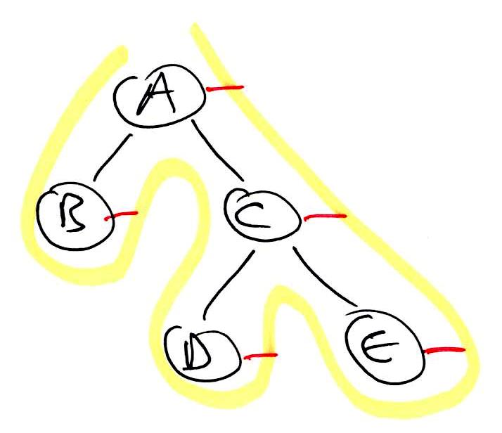
1
2
3
4
5
6
7
8  

binaryTreeTraversal(node):
    preorder(node)
    if left != null:
        binaryTreeTraversal(left)
    inorder(node)
    if right != null:
        binaryTreeTraversal(right)
    postorder(node)

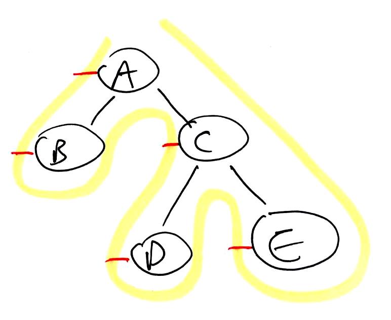
1
2
3
4
5
6
7  

Use STACK as fringe.
Add root to fringe.

while fringe not empty:
    Remove next from fringe.
    Add its children to fringe.
    Process removed node.

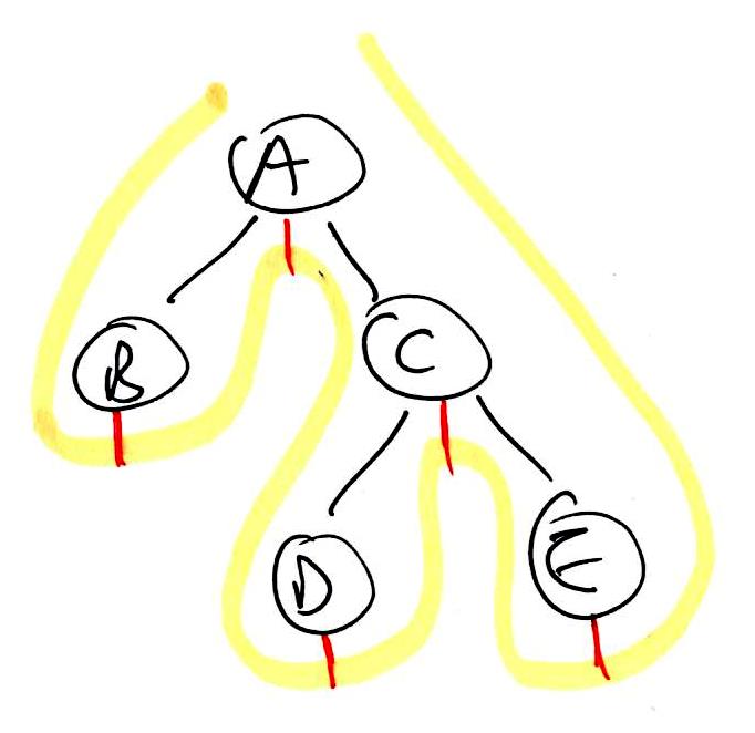
1
2
3
4
5
6
7  

Use QUEUE as fringe.
Add root to fringe.

while fringe not empty:
    Remove next from fringe.
    Add its children to fringe.
    Process removed node.

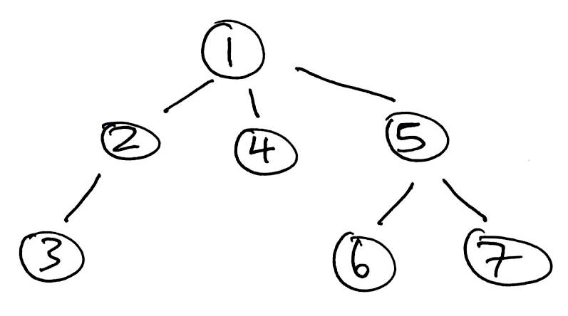
 1
 2
 3
 4
 5
 6
 7
 8
 9
10
11
12
13
14
15
16
17
18
19
20
21
22
23
24
25
26  

public BinaryTree(ArrayList<T> pre,  ArrayList<T> in) {
    root = listHelper(pre, in);
}

private TreeNode listHelper(ArrayList<T> pre,  ArrayList<T> in) {
    if (pre.isEmpty())
        return null;

    TreeNode subtreeRoot = new TreeNode(pre.get(0));

    int rootIndex = in.indexOf(pre.get(0));

    subtreeRoot.left =
            listHelper(
                    new ArrayList<>(pre.subList(1, rootIndex + 1)),
                    new ArrayList<>(in.subList(0, rootIndex))
            );

    subtreeRoot.right =
            listHelper(
                    new ArrayList<>(pre.subList(rootIndex + 1, pre.size())),
                    new ArrayList<>(in.subList(rootIndex + 1, in.size()))
            );

    return subtreeRoot;
}

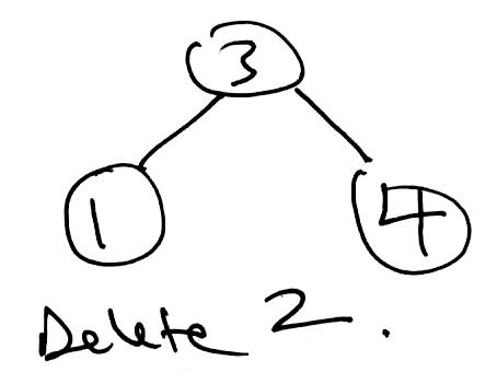
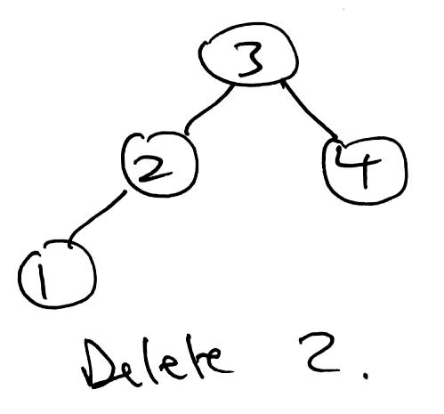
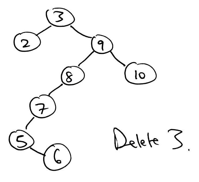
 1
 2
 3
 4
 5
 6
 7
 8
 9
10
11
12
13
14
15
16
17
18
19
20
21
22
23
24
25
26
27
28
29
30
31
32
33
34
35
36
37
38
39
40
41
42
43
44
45
46
47
48
49
50
51
52
53
54
55
56
57
58
59
60
61
62
63
64
65
66
67
68
69
70
71
72
73
74
75
76  

public T delete(T key) {
    TreeNode parent = null;
    TreeNode curr = root;
    TreeNode delNode = null;
    TreeNode replacement = null;
    boolean rightSide = false;

    // Find node to be removed.
    while (curr != null && !curr.item.equals(key)) {
        if (((Comparable<T>) curr.item).compareTo(key) > 0) {
            parent = curr;
            curr = curr.left;
            rightSide = false;
        } else {
            parent = curr;
            curr = curr.right;
            rightSide = true;
        }
    }
    delNode = curr;

    // Target was not found.
    if (curr == null) {
        return null;
    }

    // Only has a left child. Remove target and let this take its place.
    if (delNode.right == null) {
        if (root == delNode) {
            root = root.left;
        } else {
            if (rightSide) {
                parent.right = delNode.left;
            } else {
                parent.left = delNode.left;
            }
        }
    // Either has two children or just a right child.
    } else {
        curr = delNode.right;
        replacement = curr.left;

        // There was only a right child. Remove target and let this take its place.
        if (replacement == null) {
            replacement = curr;
        // There were two children.
        } else {
            // Find inorder successor replacement.
            // Leftmost node of target's right child.
            while (replacement.left != null) {
                // curr is the parent of replacement.
                curr = replacement;
                replacement = replacement.left;
            }
            // replacement does not have a left child.
            // remove replacement by letting its right child take its place.
            curr.left = replacement.right;

            // replacement takes delNode's place.
            replacement.right = delNode.right;
        }
        // replacement takes delNode's place.
        replacement.left = delNode.left;
        if (root == delNode) {
            root = replacement;
        } else {
            if (rightSide) {
                parent.right = replacement;
            } else {
                parent.left = replacement;
            }
        }
    }
    // return value of delNode.
    return delNode.item;
}

 1
 2
 3
 4
 5
 6
 7
 8
 9
10
11
12
13
14
15
16
17
18
19
20
21
22
23
24
25  

public T getKthValue(int k) {
    return getKthValueHelper(k, root);
}

private T getKthValueHelper(int k, TreeNode node) {
    if (node == null)
        return null;

    if (k >= node.size || k < 0)
        throw new IndexOutOfBoundsException();

    int numOnLeft;
    if (node.left != null)
        numOnLeft = node.left.size;
    else
        numOnLeft = 0;

    if (k < numOnLeft) {
        return getKthValueHelper(k, node.left);
    } else if (k == numOnLeft) {
        return node.item;
    } else {
        return getKthValueHelper(k - 1 - numOnLeft, node.right);
    }
}

 1
 2
 3
 4
 5
 6
 7
 8
 9
10
11  

Use STACK as fringe.
Maintain SET of visited vertices.
Add start vertex to fringe.

while fringe not empty:
    Remove next from fringe.
    if not visited:
        Process removed node.
        for each neighbor:
            Add to fringe.
        Mark removed node as visited.

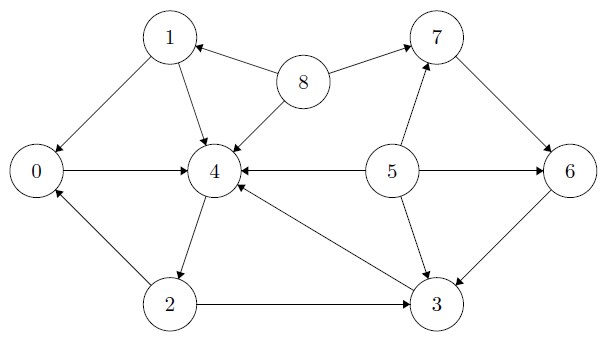
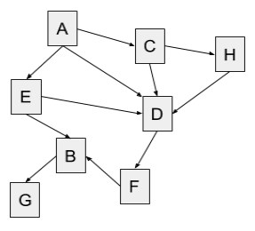
 1
 2
 3
 4
 5
 6
 7
 8
 9
10 

Maintain a FRINGE.
Maintain ARRAY of current in-degrees of all vertices.
Add in-degree 0 vertices to fringe.

while fringe not empty:
    Remove next from fringe.
    Process removed node.
    for each neighbor:
        Decrement its current in-degree.
    Add to fringe all new in-degree 0 vertices.

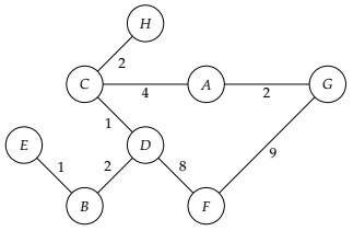
 1
 2
 3
 4
 5
 6
 7
 8
 9
10
11
12
13
14  

Use PRIORITY QUEUE as fringe.
Maintain SET of visited vertices.
Remember shortest paths to each vertex found so far.

Add start vertex to fringe.

while fringe not empty:
    Remove next from fringe.
    Mark as visited.
    The shortest path to the removed vertex has now been finalized.

    for each neighbor:
        if not visited && (shortest path to removed vertex + distance from removed vertex to neighbor) < current shortest path to neighbor:
            Either add to fringe or if already in fringe, update current shortest path to neighbor.

1
2
3
4
5 

<body>
    <h1>Oolong</h1>
    <a href=”www.earl-gray.io”>50% sugar, less ice</a>
    <center><b>Pumpkin Spice Latté</b></center>
</body>